
Triangulation from image with one connected component (proposed to F. Hecht and G. Sadaka)
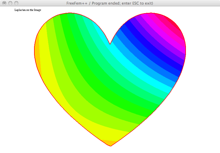
Be aware that labels are not well computed and you better look at the mesh file before doing something that needs labels. Once the triangulation is obtained, the formulation is solved on the domain defined by the image \(\Omega\):
\begin{align} -\Delta u+u & = xy,&&\text{on \(\Omega\)}\\ \partial_{n}u &=0,&& \text{on \(\partial\Omega\)} \end{align}
 |  |  |
| jpg file | Figure | Solution |
download example: ImageTriangulationOneCurve.edp or return to main page
load "isoline"

/* Chesapeake bay: Build mesh
  ----------------------------------
  made during the European Finite Element Fair 2009 in TTK/ Helsinki  (6 june 2009)
  http://math.tkk.fi/numericsyear/fefair/
  By F. Hecht
*/

load "ppm2rnm"
/*
 to bluid pgm file on shell do: # convert filename.jpg filename.pgm
*/
real[int,int] Curves(3,1);
int[int] be(1);
int nc;// nb of curve
{
string rio;

rio="baie6.pgm";
rio="a.pgm";
//rio="freefem.pgm";

real[int,int] ff1(rio); // read  image and set to an rect. array
//  remark (0,0) is the upper, left corner.
int nx = ff1.n, ny=ff1.m;
// build a cartesain mesh such that the origne is at the right place.
mesh Th=square(nx-1,ny-1,[(nx-1)*(x),(ny-1)*(1-y)]);
mesh Tf=Th;
// warning  the numbering is of the vertices (x,y) is
// given by $  i = x/nx + nx* y/ny $
fespace Vh(Th,P1);

Vh f1; f1[]=ff1;
real vmax = f1[].max ;
real vmin = f1[].min ;
real vm = (vmin+vmax)/2;
verbosity=3;
/*
 Usage of isoline
 the named parameter :
 iso=0.25        // value of iso
 close=1,        //   to force to have closing curve ...
 beginend=be,    // begin  and end of curve
 smoothing=.01,  //   nb of smoothing process = size^ratio * 0.01
 where  size is the size of the curve ...
 ratio=0.5
 file="filename"

 ouptut: xx, yy  the array of point of the iso value

a closed curve  number n is

in fortran notation the point of the curve are:
(xx[i],yy[i], i = i0, i1)
with :  i0=be[2*n],  i1=be[2*n+1];
*/

  nc=isoline(Th,f1,iso=vm,close=0,Curves,beginend=be,smoothing=.005,ratio=0.1);
  verbosity=1;
}

int ic0=be(0), ic1=be(1)-1;

macro GG(i)
border G#i(t=0,1)
{
  P=Curve(Curves,be(i*2),be(i*2+1)-1,t);
  label=i+1;
}
real lg#i=Curves(2,be(i*2+1)-1);  // END OF MACRO

// For the FreeFem ++ image use these lines because there are 6 closed curves:
// GG(0)  GG(1)	GG(2)	GG(3)	GG(4) 	GG(5)// number of closed curves
// For the heart image and the baie6 image use this line because there is only one closed curve:
GG(0)  // number of closed curves

real hh= -10;

// For the FreeFem ++ image, use these lines because there are 6 closed curves:
// func bord = G0(lg0/hh)+G1(lg1/hh)+G2(lg2/hh)+G3(lg3/hh)+G4(lg4/hh)+G5(lg5/hh);
// For the heart image and the baie6 image, use this line because there is only one closed curve:
func bord = G0(lg0/hh);

plot(bord,wait=0);
mesh Th=buildmesh(bord);
plot(Th,wait=0);
Th=adaptmesh(Th,5.,IsMetric=1,nbvx=1e6);
plot(Th,wait=0);
fespace Vh(Th,P1);

Vh u,v;

solve Problem1(u,v)=int2d(Th)(dx(u)*dx(v)+dy(u)*dy(v)+u*v)+int2d(Th)(-x*y*v);

plot(u,cmm="Laplacian on the Image ",wait=0,fill=1);
return to main page