
In this example mesh adaptation is performed to capture the function
that has a very sharp front. Visualization is made with plot and medit, error f-fh is computed and plotted according to each new mesh.
 | 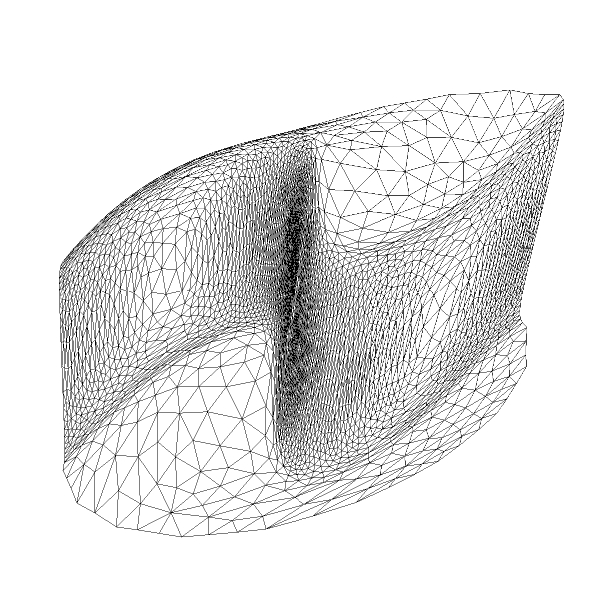 |  |
| Surface z=f(x,y) | 3D view of the mesh | Function and final mesh |
download example: aaa-adp.edp or return to 2D examples
real eps =  0.0001;
real h=1;
real hmin=0.000005;
real val=10;
real coef=50; // err = 1/100
int nbiter=6,firstplot=3;
func f = y*x*x+y*y*y+h*tanh(val*(sin(5.0*y)-2.0*x));

cout << atanh(1) << endl;
func fx = .0*y*x-0.2E1*h*(1.0-pow(tanh(val*(sin(0.5E1*y)-0.2E1*x)),2.0))*val;
func fy =  x*x+3.0*y*y+0.5E1*h*(1.0-pow(tanh(val*(sin(0.5E1*y)-0.2E1*x)),2.0))*val*cos(0.5E1*y);

func  fxy =   2.0*(x*pow(cosh(val*sin(5.0*y)-2.0*val*x),3.0)+10.0*h*val*val*cos(5.0*y)
		   *sinh(val*sin(5.0*y)-2.0*val*x))/pow(cosh(val*sin(5.0*y)-2.0*val*x),3.0);

func  fxx= 2.0*(y*pow(cosh(val*sin(5.0*y)-2.0*val*x),3.0)-4.0*h*val*val
		*sinh(val*sin(5.0*y)-2.0*val*x))/pow(cosh(val*sin(5.0*y)-2.0*val*x),3.0);

func  d = fx*fy - fxy*fxy;
func  fyy=(6.0*y*pow(cosh(val*sin(5.0*y)-2.0*val*x),3.0)-50.0*h*val*val*
	   pow(cos(5.0*y),2.0)*sinh(val*sin(5.0*y)-2.0*val*x)-25.0*h*val*sin(5.0*y)*cosh(val*
           sin(5.0*y)-2.0*val*x))/pow(cosh(val*sin(5.0*y)-2.0*val*x),3.0);

border cercle(t=0,2*pi){ x=cos(t);y=sin(t);}
mesh Th=buildmesh(cercle(20));

fespace Ph(Th,P0);
fespace Vh(Th,P1);
fespace V2h(Th,P2);
Vh fh=f;
plot(fh,wait=0); //

for (int i=0;i<nbiter;i++)
{
  //  Th=adaptmesh(Th,f);
  verbosity=4;
  Vh fxxh=fxx, fxyh=fxy, fyyh = fyy;
  cout << " min max f_xx :  " <<  fxxh[].min << " " << fxxh[].max << endl;
  cout << " min max f_yy :  " <<  fyyh[].min << " " << fyyh[].max << endl;
  cout << " min max f_xy :  " <<  fxyh[].min << " " << fxyh[].max << endl;
  Th=adaptmesh(Th,fxx*coef,fxy*coef,fyy*coef,IsMetric=1,nbvx=10000,hmin=hmin,ratio  = 5,
	       nbsmooth = 0, omega = 1);
  fh=f;
  Ph e=log10(abs(fh-f));
  Vh dh=(d>0)*2-1;
  plot(Th,fh,dh);
  real[int] vviso(20);
  for (int i=0;i<20;i++)
    vviso[i]=(-20+i)/2.;
  cout << " min max fh " << fh[].min << " " << fh[].max << endl;
  cout << " min max log(e) " << e[].min << " " << e[].max << endl;

  if (i>=firstplot)
    {
      plot(e,fill=1,value=1,wait=0,viso=vviso,cmm="log10(e) err="+1./coef);
      savemesh(Th,"Thh"+i+".mesh");
      savemesh(Th,"Th"+i,[x,y,fh/2]);
      {
        Vh eh=e;
	ofstream file("Th"+i+".BB");
	file << "2 1 1 "<< fh[].n << " 2 \n";
	int j;
	for (j=0;j<fh[].n ; j++)  {
	  file << eh[][j] << endl; }
      }
      exec("ffmedit `pwd`/Th"+i);
    }
}
return to 2D examples